Introduction

The point of sensitivity analysis is to determine how sensitive our equation is to a change in the variables. In addition, it shows which variable the equation is most sensitive to. This is done by choosing a baseline value for each variable as well as low and high values. Then the equation is analyzed one variable at a time using the low, medium, and high values, while keeping all other values at the medium value.

Methodology

Because we performed 10 trials keeping all variables the same for each plane, we did not assume a normal distribution. To conduct sensitivity analysis, low, medium, and high values had to be chosen. The values selected for the total number of frames came from the results of our experiment, with medium being the average of all our trials, low being the lowest value measured and high being the highest measured. The reference area came from the different measured areas of each plane including their flap angles with low as the 0° flap angle, medium as the 30° flap angle, and high as the 90° flap angle. The air density and drag coefficients were looked up online and the low and medium values were estimated keeping in mind what the variables would be in different environments.

GOALS OF

ANALYSIS

The purpose of performing various forms of analysis on the data we have collected is to better understand why we received the results that we did and to use that knowledge to extrapolate and draw more conclusions from. The analysis will help us to address our project hypothesis in a numerical and methodical way. Our first form of analysis is Regression and Correlation. This analysis allows us to determine how strongly different variables interact with our output, and also allows us to model our data with a simple trend line for predictions and estimates. Our second analysis method is Statistical Analysis, which uses ANOVA tests, T-Tests, and confidence intervals to find where changes in variables produce statistically different output results. This allows us to better pinpoint a specific variable value that may be statistically different from the remainder. Lastly, we used Sensitivity Analysis to discover the variables that most readily affect the output in an important way. All three analysis processes are important in drawing a final conclusion and gaining knowledge from this experiment.

Introduction:

The purpose of regression and correlation analysis is to figure out if there are relationships between mass, drag, flap angle, distance and velocity. If there is a relationship, we will figure out if it is true, as well as find out how strong or weak the relationship is. We will examine: Distance vs. Flap Angle, Drag vs. Flap Angle, Distance vs. Mass, and Drag vs. Mass.

Methodology:

The procedure was to first graph the data points of the relationship we were examining in Excel as well as their averages. From here we were about to find a trend line, see how well it fit, and figure out if it logically made sense. Also in Excel, we calculated the correlation coefficient to see if there was an overall positive or negative trend. Last we described why we think there was a trend in the cases that there were.

SENSITIVITY ANALYSIS

By: Conner Reyer

Results

Distance vs. flap angle

Correlation Coefficient: 0.708

For Distance vs. Flap Angle, we took 10 trials with the rear elevator flaps at 0˚, 30˚, 60˚, and 90˚. These trials were then averaged which you can see on the graph (Figure 19). When analyzing Distance vs. Flap Angle for normal copy paper, no correlations could be concluded. No type of trend line or equation could reasonably explain the variation in the data. There is however an overall, moderately strong, positive trend, which can be seen by the correlation coefficient below.

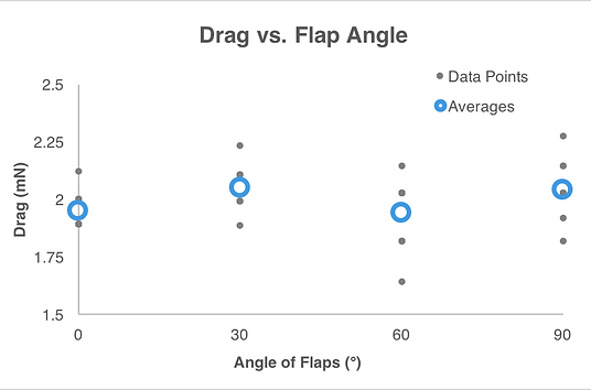
Drag vs. Flap angle

Correlation Coefficient: 0.356

For Drag vs. Flap Angle we again took 10 trials and averaged them. To calculate drag we used the above equation. As can be see by the graph to the left (Figure 20), there is no correlation between drag and flap angle. No equation can relate the two variables together. There is also barely any positive correlation overall as the correlation coefficient below is very small.

Distance vs. Mass

For Distance vs. Mass, there was a strong negative correlation, as can be seen below with the correlation coefficient. There was a linear trend with the equation of :

Correlation Coefficient: -0.978

Distance = -0.014 × Mass + 1.467

With the high coefficient of regression of 0.957, see Figure 21, we can conclude that the trend line fits the data very well. We believe that the distance decreased as mass increased because the heavier plane had a smaller lift force in comparison to the force of gravity. This caused the upward force to be relatively smaller. Therefore, the heavier the plane, the sooner it will hit the ground.

Drag Vs. Mass

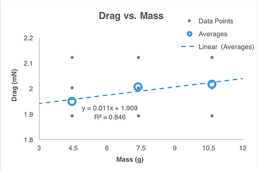
For Drag vs. Mass, there was a strong positive correlation, which can be seen by the correlation coefficient below. There was a linear trend with the equation of :

Drag = 0.011 × Mass + 1.909

This equation fit the data relatively well, see Figure 22, with a coefficient of regression of 0.846. We believe that the drag increased as mass increased since the higher mass planes had a higher momentum and had a higher speed for longer. This higher speed would increase the drag that we calculated. We took this study a step further and compared velocity and mass as mass increased. This graph can be seen below and supports our hypothesis (see Figure 23).

Correlation Coefficient: 0.920

Correlation Coefficient: 0.921

The Velocity vs. Mass graph, Figure 23, supports our hypothesis since the velocity increases with mass. Both the correlation coefficient (below) and the coefficient of regression (on figure 23) show a strong positive correlation. We can conclude through this that the increased momentum caused the plane to hold it's higher velocity for a longer time, and therefore have a higher force of drag.

Figure 19: This graph shows all of the total distances for the 4 different flap angles, as well as the average for each angle. There is no correlation.

Figure 20: This graph shows the Drag calculated for each of the 10 trials for the 4 different flap angles, as well as the average for each angle. There is no correlation.

Figure 21: This graph shows the Distance for each of the 10 trials for the 3 different paper types (normal, construction, cardstock). It also shows the average for each mass. There is a strong negative, linear correlation that can be seen on the graph.

Figure 22: This graph shows the calculated Drag for each of the 10 trials for the 3 different paper types (normal, construction, cardstock). It also shows the average for each mass. There is a strong positive, linear correlation that can be seen on the graph.

Figure 23: This graph shows the average velocity over the first 50 cm for each of the 10 trials for the 3 different paper types (normal, construction, cardstock). It also shows the average for each mass. There is a strong positive, linear correlation that can be seen on the graph.

Anchor 1

Regression and Correlation

By: Vaughn Chambers

Analysis

INTRODUCTION

The purpose of using ANOVA, T-Tests, and Confidence Intervals is to determine if the distance traveled by the planes and/or the drag force was significantly different with a certain elevator flap angle or paper mass used in the design.

METHODS

Because of our small sample size of 10 trials per plane setup (paper material and flap angle), we needed to utilize t-tests. To make more efficient use of time analyzing the data, ANOVA tests were conducted to find if there were any significant differences between drag and distance values from each trial set. If a significant difference was found, t-tests were later performed to find out the exact parameters that caused significant differences in the data. The averages of the data from each parameter were also graphed with error bars showing 95% confidence of where each mean lies. This provides a clear visual representation of how the results change across the data sets.

RESULTS

DISTANCE Vs. Mass

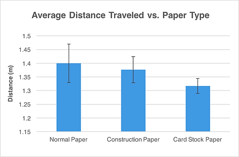
To determine if the mass of the paper used to build the paper airplane provided significant difference in the distance traveled, an ANOVA test was run. As can be seen in Table 11, the ANOVA test showed a p value of 0.081, which is above our threshold of a = 0.05. Thus, we cannot be confident that any mass of paper leads to statistically different distances traveled by the paper airplane.

However, an interesting relation can be seen in the confidence intervals. It seems as mass increased, the spread of the data decreased, see Figure 24. This is a neat finding that indirectly shows that the lift force with respect to gravitational force becomes more negligible as mass increases.

Table 11: ANOVA test of Distance vs. Mass

DISTANCE VS. FLAP ANGLE

Based on the ANOVA and T-Tests, we can have good reason to believe that varying the planes’ elevator flap angle significantly changes the distance that the plane travels. T-Tests show significance between all flap angles, except for between 30˚ and 60˚, which did not show enough difference in data to be statistically significant (based on a = 0.05). This provides interesting information that could lead to a better understanding of what factors are most helpful in a paper airplane flying for distance.

It seems that at a level release angle and consistent release velocity, a 30˚ flap angle will yield the farthest distances traveled. The 30˚ angle is closely followed by 60˚ and 90˚, however a 0˚ shows significantly lower distance values when compared to the data from the remaining flap angles. This information can be seen in the Excel sheets as well as in the graphs in Table 12 and Figure 25 .

Table 12: ANOVA test of Distance vs. Flap Angle

DRag VS. MASS

The ANOVA test yielded no statistical significance between the different paper masses and the drag of the paper airplane. As seen in Table 13, the ANOVA test produced a p value of 0.189, which is far above our threshold. Given this information, we do not have sufficient evidence to claim that the drag force is significantly affected by the change in the mass of paper used. This information can be seen graphically in Figure 26.

Table 13: ANOVA test of Drag vs. Mass

DRag VS. FLAP ANGLE

The last ANOVA test performed was to test the statistical significance of the flap angles vs. the drag force on the plane. Once again, this ANOVA test showed no statistically significant difference with a p value of 0.064 (Table 14). Due to this, we could not reject the null, meaning that we could not claim that differing flap angles have an effect on the drag force. This is slightly concerning since the distance was affected, however the drag did not have enough statistical evidence to assume the same. This means that the distance must have been mainly affected by some other element, such as lift. Figure 27 shows this data graphically.

Figure 25: Graph showing how flap angle affects the average distance traveled by the plane during a trial set.

Figure 26: Graph showing how paper type affects the average drag force on the plane during a trial set.

Table 14: ANOVA test of Drag vs. Flap Angle

Figure 27: Graph showing how flap angle affects the average drag force on the plane during a trial set.

Figure 24: Graph showing how paper mass affects the average distance traveled by the plane during a trial set.

CONCLUSION:

From these ANOVA and T-Tests, we can say with 95% confidence that flap angle has an effect on the distance traveled by the plane. Essentially, if longer travelling distance is desired in a plane design, a flap angle of 30˚, 60˚, or 90˚ would be needed. All are statistically different from each other, except for 30˚ and 60˚, however they all enable much farther travel when compared relatively to a flap angle of 0˚.

Statistical Analysis EXCEL WORKBOOK:

Conclusion:

From this analysis, we have concluded that Flap Angle did not correlate with neither Drag nor Distance. We were not able to find any kind of relationship for either of these other than both of them having a moderately strong correlation coefficient, and thus having an overall positive trend. However, there was a relationship between Mass and Distance. We found that as Mass increases, Distance linearly decreases. We believe this is due to a heavier plane having a smaller relative lift force, and therefore falling faster. Mass also correlated to Drag, as Drag increased with an increasing Mass. After further analysis we found that this was due to a heavier plane having a higher momentum and retaining more of it's initial speed over a longer period. We found that as plane mass increased, the planes would travel faster but do so on a more downward path causing a decrease in total distance.

Regression and Correlation Excel Workbook:

STATISTICAL ANALYSIS

By: Lake Bender

Results

The sensitivity analysis was done on our equation for drag. The low, medium, and high values selected are shown in Table 15. While it is obvious from our equation that the drag coefficient and air density will have the greatest effect, we cannot control those variable. Of the variables we can control, we expect the drag equation will be most sensitive to the total number of frames between take off and crossing the half meter mark as this is how we calculated our velocity. A sample calculation is shown in Table 15.

After graphing the sensitivity analysis (Figure 28), it is easy to see that the drag coefficient and the total number of frames have the biggest impact on change in drag. While all variables do have some impact, the reference area does not seem to affect our findings very greatly. The drag coefficient does account for the largest amount of change, as we expected, with the total number of frames as a close second.

Taking each drag found and dividing it by our medium value in Table 15 produced a percentage showing the change that was generated by altering the particular variable. This graph (Figure 29) also shows that the drag coefficient causes the largest change in drag as the coefficient rises. Additionally, the graph displays how the overall equation changes as each variable increases. As you can see, the drag coefficient and air density increase greatly, while the reference area increases slightly. Total frames, in contrast, causes a significant decrease.

Variable Values

Graphs

Figure 28: This graph shows how the drag force changed as one variable was changed and the rest remained at their medium value.

Figure 29: This graph shows how much % off the baseline the drag is when one variable is changed.

Table 15: This chart shows the low, medium and high values for each variable, as well as the baseline drag value. Note that the Area takes into account the changing flap angle.

Conclusion

In conclusion, the drag equation we used is most sensitive to the drag coefficient and the air density. Because we cannot control these variables, however, they do not provide us with helpful information. It was found that the increase in total number of frames between take off and the half meter mark caused a significant reduction in drag. As the number of frames rose the overall velocity of the plane decreased, causing a decrease in drag force. This matches our project hypothesis that the drag is proportional to the velocity squared. With very little sensitivity due to the reference area it is hard to say for certain that changing the flap angle of the plane affects the plane’s flight. Overall, the sensitivity analysis did show the proportionality of drag to velocity but did not show with as great a change the influence of the flap angle.

Sensitivity Analysis Excel Workbook: